41 add data labels to the best fit position

Display data point labels outside a pie chart in a paginated report ... To display data point labels inside a pie chart. Add a pie chart to your report. For more information, see Add a Chart to a Report (Report Builder and SSRS). On the design surface, right-click on the chart and select Show Data Labels. To display data point labels outside a pie chart. Create a pie chart and display the data labels. Open the ... Excel VBA Code for data label position - MrExcel Message Board If you select 'Format Data Labels' using the right-click context menu on a label, the properties pane on the right hand side only has 'Centre', 'Inside End' and 'Inside Base' for column charts (for example). As I want to move a column label above the column I suspect I'm going to have to move it to an absolute position .

Improve your X Y Scatter Chart with custom data labels Go to tab "Insert". Press with left mouse button on the "scatter" button. Press with right mouse button on on a chart dot and press with left mouse button on on "Add Data Labels". Press with right mouse button on on any dot again and press with left mouse button on "Format Data Labels". A new window appears to the right, deselect X and Y Value.

Add data labels to the best fit position

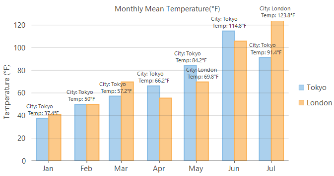
Excel 2010 pie chart data labels in case of "Best Fit" Based on my tested in Excel 2010, the data labels in the "Inside" or "Outside" is based on the data source. If the gap between the data is big, the data labels and leader lines is "outside" the chart. And if the gap between the data is small, the data labels and leader lines is "inside" the chart. Regards, George Zhao TechNet Community Support How to find, highlight and label a data point in Excel scatter plot Select the Data Labels box and choose where to position the label. By default, Excel shows one numeric value for the label, y value in our case. To display both x and y values, right-click the label, click Format Data Labels…, select the X Value and Y value boxes, and set the Separator of your choosing: Label the data point by name Format Data Labels in Excel- Instructions - TeachUcomp, Inc. To do this, click the "Format" tab within the "Chart Tools" contextual tab in the Ribbon. Then select the data labels to format from the "Chart Elements" drop-down in the "Current Selection" button group. Then click the "Format Selection" button that appears below the drop-down menu in the same area.

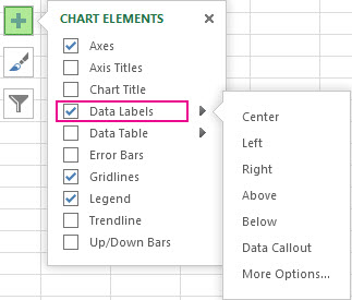
Add data labels to the best fit position. Excel charts: add title, customize chart axis, legend and data labels ... To add a label to one data point, click that data point after selecting the series. Click the Chart Elements button, and select the Data Labels option. For example, this is how we can add labels to one of the data series in our Excel chart: For specific chart types, such as pie chart, you can also choose the labels location. Office: Display Data Labels in a Pie Chart - Tech-Recipes 1. Launch PowerPoint, and open the document that you want to edit. 2. If you have not inserted a chart yet, go to the Insert tab on the ribbon, and click the Chart option. 3. In the Chart window, choose the Pie chart option from the list on the left. Next, choose the type of pie chart you want on the right side. 4. Position labels in a paginated report chart - Microsoft Report Builder ... On the design surface, right-click the chart and select Show Data Labels. Open the Properties pane. On the View tab, click Properties On the design surface, click the series. The properties for the series are displayed in the Properties pane. In the Data section, expand the DataPoint node, then expand the Label node. VBA Bestfit position for datalabels on line chart - Stack Overflow "Best fit" is a setting unique to pie chart data labels. You have the option of positioning a line chart's data labels centered (directly on a point), as well as above, below, left of, and right of the point. You can also position the data label anywhere by changing the .left and .top properties of the label.

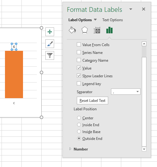
How to Customize Your Excel Pivot Chart Data Labels - dummies To add data labels, just select the command that corresponds to the location you want. To remove the labels, select the None command. If you want to specify what Excel should use for the data label, choose the More Data Labels Options command from the Data Labels menu. Excel displays the Format Data Labels pane. Create Dynamic Chart Data Labels with Slicers - Excel Campus Step 6: Setup the Pivot Table and Slicer. The final step is to make the data labels interactive. We do this with a pivot table and slicer. The source data for the pivot table is the Table on the left side in the image below. This table contains the three options for the different data labels. Change the format of data labels in a chart To get there, after adding your data labels, select the data label to format, and then click Chart Elements > Data Labels > More Options. To go to the appropriate area, click one of the four icons ( Fill & Line, Effects, Size & Properties ( Layout & Properties in Outlook or Word), or Label Options) shown here. Add or remove data labels in a chart - support.microsoft.com To label one data point, after clicking the series, click that data point. In the upper right corner, next to the chart, click Add Chart Element > Data Labels. To change the location, click the arrow, and choose an option. If you want to show your data label inside a text bubble shape, click Data Callout.

Creating Pie Chart and Adding/Formatting Data Labels (Excel) Creating Pie Chart and Adding/Formatting Data Labels (Excel) Fit Chart Labels Perfectly in Reporting Services using Two ... - Doug Lane Make the labels smaller. Move or remove the labels. Option #1 gets ruled out frequently for information-dense layouts like dashboards. Option #2 can only be used to a point; fonts become too difficult to read below 6pt (even 7pt font can be taxing to the eyes). Option #3 - angled/staggered/omitted labels - simply may not meet our needs. How to add or move data labels in Excel chart? - ExtendOffice 2. Then click the Chart Elements, and check Data Labels, then you can click the arrow to choose an option about the data labels in the sub menu. See screenshot: In Excel 2010 or 2007. 1. click on the chart to show the Layout tab in the Chart Tools group. See screenshot: 2. Then click Data Labels, and select one type of data labels as you need ... Data Labels in Power BI - SPGuides To format the Power BI Data Labels in any chart, You should enable the Data labels option which is present under the Format section. Once you have enabled the Data labels option, then the by default labels will display on each product as shown below.

Move data labels - Office Support

Custom Excel Chart Label Positions - My Online Training Hub A solution to this is to use custom Excel chart label positions assigned to a ghost series. For example, in the Actual vs Target chart below, only the Actual columns have labels and it doesn't matter whether they're aligned to the top or base of the column, they don't look great because many of them are partially covered by the target column:

How-to: Analyze documents, Label forms, train a model, and analyze forms with Form Recognizer ...

Excel Charts: Dynamic Label positioning of line series - XelPlus Select your chart and go to the Format tab, click on the drop-down menu at the upper left-hand portion and select Series "Budget". Go to Layout tab, select Data Labels > Right. Right mouse click on the data label displayed on the chart. Select Format Data Labels. Under the Label Options, show the Series Name and untick the Value.

How to Add Data Labels to an Excel 2010 Chart - dummies On the Chart Tools Layout tab, click Data Labels→More Data Label Options. The Format Data Labels dialog box appears. You can use the options on the Label Options, Number, Fill, Border Color, Border Styles, Shadow, Glow and Soft Edges, 3-D Format, and Alignment tabs to customize the appearance and position of the data labels.

Data Labels | ComponentOne FlexChart for WinForms

Adding Data Labels to Your Chart - Excel ribbon tips Select the position that best fits where you want your labels to appear. To add data labels in Excel 2013 or Excel 2016, follow these steps: Activate the chart by clicking on it, if necessary. Make sure the Design tab of the ribbon is displayed. (This will appear when the chart is selected.) Click the Add Chart Element drop-down list.

ios - Pinning a view to the bottom with dynamic height - Stack Overflow

Apply Custom Data Labels to Charted Points - Peltier Tech Click once on a label to select the series of labels. Click again on a label to select just that specific label. Double click on the label to highlight the text of the label, or just click once to insert the cursor into the existing text. Type the text you want to display in the label, and press the Enter key.

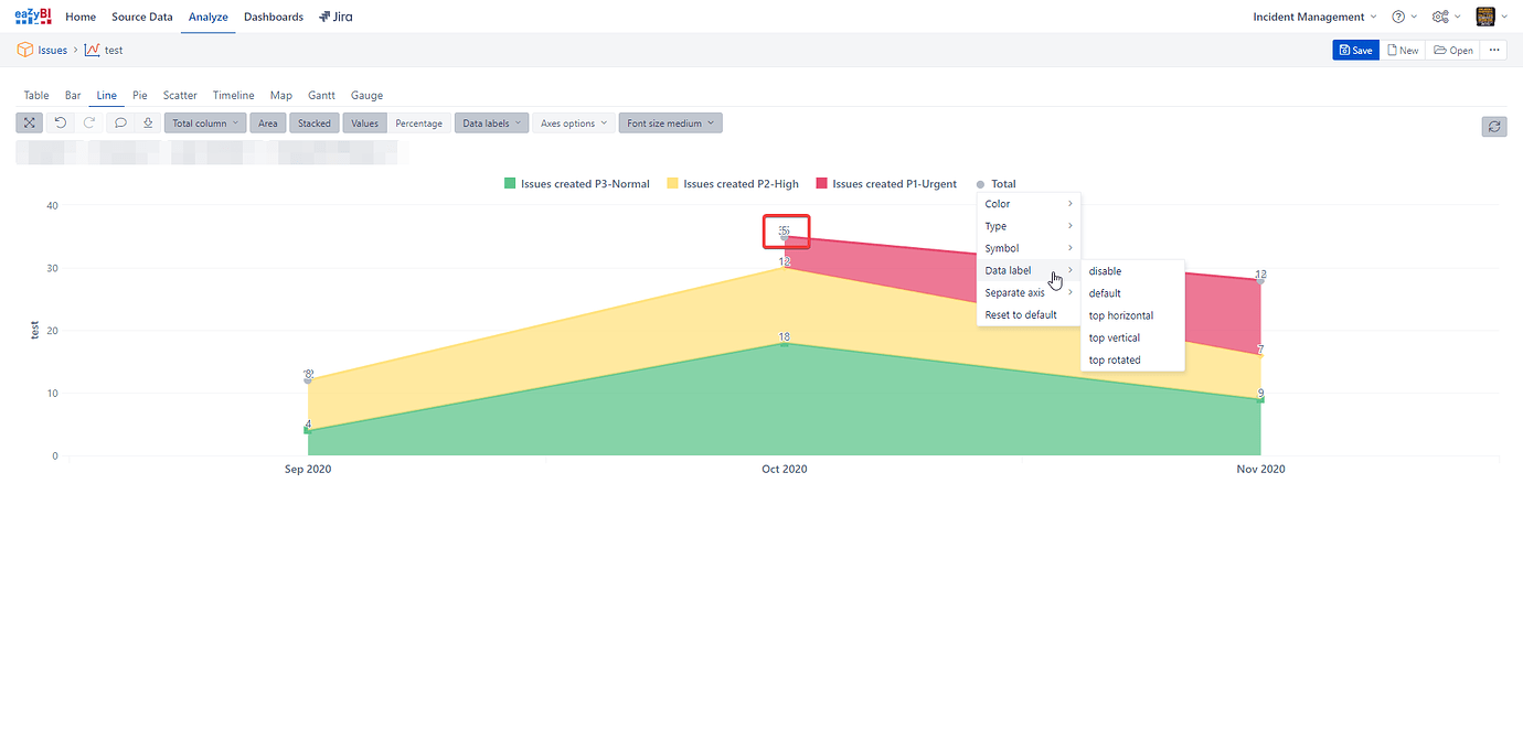
How position Data Label to avoid them to stack? - Questions & Answers - eazyBI Community

DataLabels Guide - ApexCharts.js In a multi-series or a combo chart, if you don't want to show labels for all the series to avoid jamming up the chart with text, you can do it with the enabledOnSeries property. This property accepts an array in which you have to put the indices of the series you want the data labels to appear. dataLabels: { enabled: true , enabledOnSeries ...

Format Data Label Options in PowerPoint 2013 for Windows Alternatively, select data labels of any data series in your chart and right-click to bring up a contextual menu, as shown in Figure 2, below. From this menu, choose the Format Data Labels option. Figure 2: Format Data Labels option Either of these options opens the Format Data Labels Task Pane, as shown in Figure 3, below.

Python The Complete Manual First Edition [r217149p8g23]

12.3. Setting a label — QGIS Documentation documentation 12.3.1.2. Formatting tab . Fig. 12.16 Label settings - Formatting tab . In the Formatting tab, you can:. Use the Type case option to change the capitalization style of the text. You have the possibility to render the text as: No change. All uppercase. All lowercase. Title case: modifies the first letter of each word into capital, and turns the other letters into lower case if the original text ...

javascript - How to create a dynamic amount of labels to fit with the data in chartjs? - Stack ...

Label your map—ArcGIS Pro | Documentation - Esri On the Map tab, in the Navigate group, click Bookmarks and click Historic Buildings 1. In the Contents pane, click the Building Footprints layer to select it. On the ribbon, under Feature Layer, click the Labeling tab. On the Labeling tab, in the Layer group, click Label . The buildings are labeled.

Advanced Label Data

Format Data Labels in Excel- Instructions - TeachUcomp, Inc. To do this, click the "Format" tab within the "Chart Tools" contextual tab in the Ribbon. Then select the data labels to format from the "Chart Elements" drop-down in the "Current Selection" button group. Then click the "Format Selection" button that appears below the drop-down menu in the same area.

How to find, highlight and label a data point in Excel scatter plot Select the Data Labels box and choose where to position the label. By default, Excel shows one numeric value for the label, y value in our case. To display both x and y values, right-click the label, click Format Data Labels…, select the X Value and Y value boxes, and set the Separator of your choosing: Label the data point by name