43 conditional formatting data labels excel

How to Apply Conditional Formatting to Pivot Tables - Excel … 12.12.2018 · Bottom Line: Learn how to apply conditional formatting to pivot tables so that the formats are dynamically reapplied as the pivot table is changed, filtered, or updated. Skill Level: Intermediate Download the Excel File. Here's the file that I use in the video. You can use it to practice adding, deleting, and changing conditional formatting on a variety of pivot table … Excel Data Analysis - Conditional Formatting - Tutorials Point Follow the steps to conditionally format cells − Select the range to be conditionally formatted. Click Conditional Formatting in the Styles group under Home tab. Click Highlight Cells Rules from the drop-down menu. Click Greater Than and specify >750. Choose green color. Click Less Than and specify < 500. Choose red color.

Conditional Formatting in Excel - a Beginner's Guide Click Conditional Formatting, then select Icon Set to choose from various shapes to help label your data. For this example, let's use the arrow icon set to show whether our highlighted data, the Variance column, has increased or decreased. Now, you'll see that the data has arrow icons accompanying their values in the cells.

Conditional formatting data labels excel

Excel tutorial: How to add a conditional formatting key That way, we can adjust the conditions for the rules using the key itself. The first step is to create the basic layout for the key. For this, we'll set up a small table with three rows - one for each conditional format. We can then add labels for each conditional format rule. These could be anything, but let's use Excellent, Concern, and ... Can I use conditional formatting to change colors depending on data values? To set up conditional formatting, select the respective data cells in the Excel file. For line charts, the fill color of data cells controls the color of markers (see Line scheme). The line color itself is controlled by the cell containing the line series label. These cells may contain any number format, formulas, and references to other cells. VBA Conditional Formatting of Charts by Value and Label The category labels (XValues) and values (Values) are put into arrays, also for ease of processing. The code then looks at each point's value and label, to determine which cell has the desired formatting. The rows and columns are looped starting at 2, since the first of each contains an irrelevant label. The looping stops one count before the end.

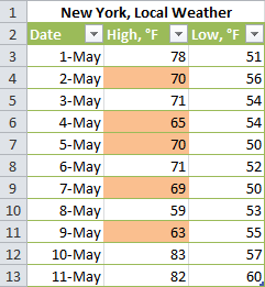
Conditional formatting data labels excel. Excel conditional formatting Icon Sets, Data Bars and Color Scales Select all cells in column A, except for the column header, and create a conditional formatting icon set rule by clicking Conditional Formatting > Icon sets > More Rules... In the New Formatting Rule dialog, select the following options: Click the Reverse Icon Order button to change the icons' order. Select the Icon Set Only checkbox. Changing the Color of a Data Label using IF Statement 1) Click on the data labels to highlight all the data labels, 2) Right-Click and select Format Data Labels, 3) Click on Number, 4) Go to the Format Code field *adapt the following to your needs* 5) [green] [>29]#.00; [<30] [Color 53]#.00 Click to expand... Hi Jawnne, I hope you're still lurking about on here. Conditional Formatting in Excel (In Easy Steps) 1. Select the range A1:A10. 2. On the Home tab, in the Styles group, click Conditional Formatting. 3. Click Highlight Cells Rules, Greater Than. 4. Enter the value 80 and select a formatting style. 5. Click OK. Result. Excel highlights the cells that are greater than 80. 6. Change the value of cell A1 to 81. Result. Use conditional formatting to highlight information Conditional formatting can help make patterns and trends in your data more apparent. To use it, you create rules that determine the format of cells based on their values, such as the following monthly temperature data with cell colors tied to cell values.

Conditional Formatting - Tableau Different than excel, conditional formatting in Tableau cannot be applied across a column but rather across a mark. Marks are generated when measures are added to the rows/columns shelf. Adding these additional marks allows a user to achieve a similar result to excel-like conditionally formatted crosstabs. See below for the steps required to ... Conditional Formatting Using Custom Measure - Power BI 28.9.2020 · Voila! We have given conditional formatting to Day of Week column based on the clothing Category value. I just tried to add a simple legend on the top to represent the color coding. So, this is how one can use a custom color formatting in Power BI by creating a simple measure for it. Hope this article helps everyone out there. - Pragati How to do conditional formatting of a label in Excel VBA Function ConditionalFormatNumber (n As Double) As String If n > 1000000 Then ConditionalFormatNumber = Format (n / 1000000, "$#,##0.00,,""M""") ElseIf n > 1000 Then ConditionalFormatNumber = Format (n / 1000, "$#,##0.00, ""K""") Else ConditionalFormatNumber = Format (n, "$#,##0.0") End If End Function Share answered Aug 24, 2017 at 9:13 Format Data Labels in Excel- Instructions - TeachUcomp, Inc. To do this, click the "Format" tab within the "Chart Tools" contextual tab in the Ribbon. Then select the data labels to format from the "Chart Elements" drop-down in the "Current Selection" button group. Then click the "Format Selection" button that appears below the drop-down menu in the same area.

Microsoft Excel conditional number formatting Sep 17, 2019 · Using custom number formatting and conditional formatting combined the requirement is fairly straightforward. My suggested solution would be: Construct the underlying number formatting first. Personally, I would use custom number formatting so that all positive and negative numbers appeared as percentages, zero as a hyphen and text as displayed ... Conditional Formatting Shapes - Step by step Tutorial Let's see step by step how to create it: First, select an already formatted cell. In the picture below, we have created a little example of this. We will pay attention to the range D5:D6. You can see the rules in the Rules Manager window. We didn't make it overly complicated. Conditional Formatting - Tableau Different than excel, conditional formatting in Tableau cannot be applied across a column but rather across a mark. ... we can start to customize the labeling and format of those rows to look just like a conditionally formatted crosstab in excel. Add separate KPIs and data labels to the respective marks cards and you achieve the final result below. Excel Conditional Formatting not functioning correctly after ... Jan 10, 2018 · Everything works fine, formatting changes according to changes in the data! Now I copy a range of sheet A to sheet B using VBA, that works OK. However: in sheet B the conditional formatting of these cells is not working correctly anymore: > cells using 'format only cells that contain' work correct! formatting changes correctly when data changes

Conditional Formatting in Excel - a Beginner's Guide

Excel Conditional Formatting Data Bars Select the cells that contain the data bars. On the Ribbon, click the Home tab. In the Styles group, click Conditional Formating, and then click Manage Rules. In the list of rules, click your Data Bar rule, then click the Edit Rule button. In the "Edit the Rule Description" section, the default settings are shown for Minimum and Maximum.

Conditional Format that Checks for Data Type (Microsoft Excel)

Conditional Formatting For Blank Cells | (Examples and Excel ... Always use limited data to deal with and apply bigger conditional formatting to avoid excel getting freeze. Recommended Articles. This has been a guide to Conditional Formatting for Blank Cells. Here we discuss how to apply Conditional formatting for blank cells along with practical examples and a downloadable excel template.

How to Create Multi-Category Chart in Excel - Excel Board

Conditional formatting for Excel column charts - Think Outside The Slide Press Ctrl+1 to open the Format Data Series task pane. Set the Series Overlap to 100% and the Gap Width to 50%. The Series Overlap layers the columns on top of each other but since there is only one visible column in each month, no data is hidden. The Gap Width settings makes the columns wider so they have more presence on the chart.

Tableau Legends Per Measure and Conditional Formatting Like Excel

Conditional formatting chart data labels? - Excel Help Forum The easy way to conditionally format these labels is use two series. Use something like =IF ($E2=1,0,NA ()) for the series that has red labels and =IF (#E2=1,NA (),0) for the series that has unformatted labels. Jon Peltier Register To Reply Bookmarks Digg del.icio.us StumbleUpon Google Posting Permissions

How to use conditional formatting in Excel

Excel Conditional Formatting not functioning correctly after … 10.1.2018 · Everything works fine, formatting changes according to changes in the data! Now I copy a range of sheet A to sheet B using VBA, that works OK. However: in sheet B the conditional formatting of these cells is not working correctly anymore: > cells using 'format only cells that contain' work correct! formatting changes correctly when data changes

How to Copy Conditional Formatting in Excel

How to Change Excel Chart Data Labels to Custom Values? 5.5.2010 · Now, click on any data label. This will select “all” data labels. Now click once again. At this point excel will select only one data label. Go to Formula bar, press = and point to the cell where the data label for that chart data point is defined. Repeat the process for all other data labels, one after another. See the screencast.

How to Create Multi-Category Chart in Excel - Excel Board

How to Apply Conditional Formatting to Pivot Tables - Excel ... Dec 12, 2018 · Conditional Formatting can change the font, fill, and border colors of cells. It can also add icons and data bars to the cells. The formatting will also be applied when the values of cells change. This is great for interactive pivot tables where the values might change based on a filter or slicer. How to Setup Conditional Formatting for Pivot ...

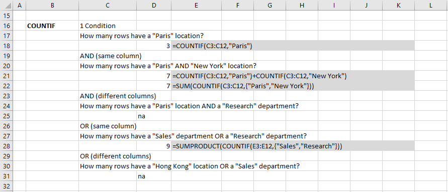
Excel Functions Conditional Counting

How to create a chart with conditional formatting in Excel? Add three columns right to the source data as below screenshot shown: (1) Name the first column as >90, type the formula =IF (B2>90,B2,0) in the first blank cell of this column, and then drag the AutoFill Handle to the whole column;

How to create progress bar chart in Excel?

Creating Conditional Data Labels in Excel Charts - YouTube We can make labels appear on our charts that don't have to do with the raw numbers that built the chart - and we can make them show up or not based on whatever conditions we want. In this tutorial,...

How to Create Multi-Category Chart in Excel - Excel Board

Excel conditional formatting highlight row based on date 1. Select the table you will highlight rows if dates have passed, and click Home > Conditional Formatting > New Rule. See screenshot: 2. In the Edit Formatting Rule dialog box, please: (3) Click the Format button. 3. In the Format Cells dialog box, go to the Fill tab, and click to select a fill color. See screenshot:

Conditional formatting using VBA macros

Conditional Formatting of Excel Charts - Peltier Tech From the Data Label options, I am able to include any of the 4 data cateogires; however, i cannot include the customer name. ... Conditional Formatting of Excel Charts - Peltier Tech Blog […] Conditional Format Chart says: Sunday, June 26, 2016 at 4:13 pm […] document.write(''); y tutorial on this topic is at Conditional Formatting of ...

Conditional Formatting of Excel Charts - Peltier Tech Blog

Identify Duplicate Values With Conditional Formatting The last option in the New Formatting Rule dialogue box is where we can get a bit more creative. Use your own custom formulas to create any number of conditional formatting rules. The Conditional Formatting must return a TRUE or FALSE or numerical equivalent. An example of some formulas that work perfectly with this type of formatting. =A2>50

[SOLVED] Conditional copying data into another sheet

Microsoft Excel conditional number formatting 17.9.2019 · Next, I would apply conditional formatting number formatting where the cell value is greater than one so that numbers greater than a million could be displayed to the nearest 0.1m, numbers less than a million but greater than or equal to 1,000 could be displayed to the nearest 0.00k and numbers lower than 1,000 (but necessarily greater than one) could be displayed as …

Docs | How to use conditional formatting in Sheets

Date Related Conditional Formatting Rules in Google Sheets 2. The same Conditional Formatting panel you can open from the Format menu. To know about how to conditional format in Google Sheets, follow the below examples. Single Cell, Entire Row and Entire Column in Conditional Formatting in Google Sheets. The Dollar Sign ($) has great importance in the Conditional formatting formulas.

excel - Conditional formatting for contains certain text from a range of values - Stack Overflow

Conditional Formatting For Blank Cells | (Examples and Excel Always use limited data to deal with and apply bigger conditional formatting to avoid excel getting freeze. Recommended Articles. This has been a guide to Conditional Formatting for Blank Cells. Here we discuss how to apply Conditional formatting for blank cells along with practical examples and a downloadable excel template.

Excel Basic Formatting

Tom’s Tutorials For Excel: Conditionally Formatting Locked and ... In the Conditional Formatting dialog box, click OK, and you are done. IF YOU ARE USING EXCEL VERSION 2007 OR AFTER: Step 5 (version 2007 or after) — Press Alt+O+D to show the Conditional Formatting Rules Manager dialog box: • In the “Show Formatting Rules for” field, select Current Selection. • Click on the item labeled “New Rule”.

[SOLVED] Conditional copying data into another sheet

How to change chart axis labels' font color and size in Excel? Sometimes, you may want to change labels' font color by positive/negative/ in an axis in chart. You can get it done with conditional formatting easily as follows: 1. Right click the axis you will change labels by positive/negative/0, and select the Format Axis from right-clicking menu. 2.

Share :